Tutorial

Check the version

./MuSTA.R -v

#> 0.0.1

Dry-run

In order to check your config file before actually processing it, the --dry-run option is useful.

./MuSTA.R \
  --dry-run \
  --input test/input.csv \
  --gtf test/reference/test.ref.gtf \
  --genome test/reference/chr16_18_head.fa

This command returns 4 types of information.

1. Valid arguments
2. Session information
3. Paths to intermediate files to be generated.
4. The generated workflow based on the options

In addition, you can find ‘plan_pre_run.pdf’ in your working directory, which visualizes the generated workflow.

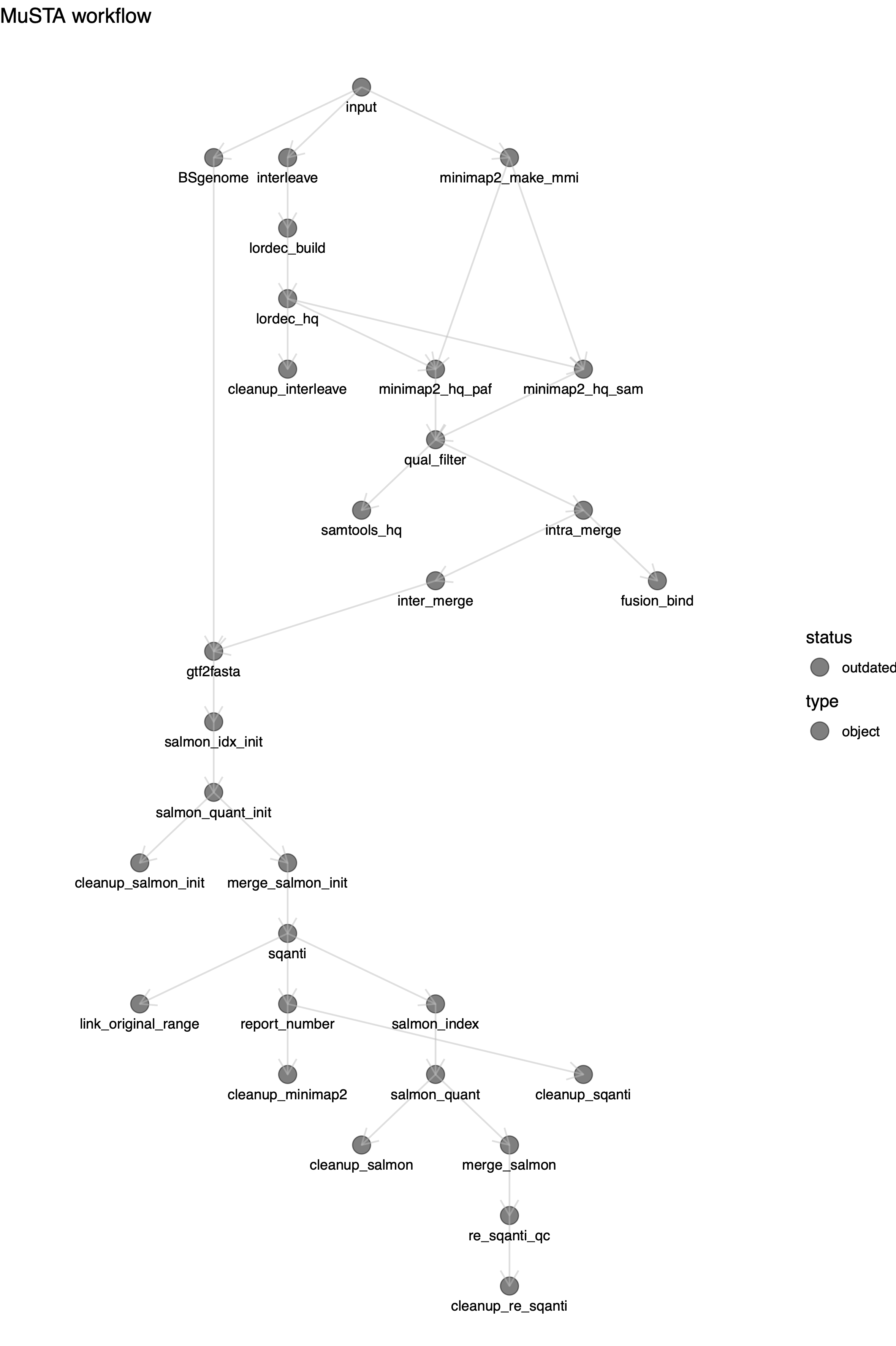plan_pre_run

Test run

You can apply MuSTA to a test data by

./MuSTA.R \
  --input test/input.csv \
  --gtf test/reference/test.ref.gtf \
  --genome test/reference/chr16_18_head.fa \
  --output test/test_output

This command creates a directory named ‘test/test_output’ containing 8 sub-directories

output:
    result
    report
    script
    log
    sample
    merge
    fusion
    genome

By checking ‘report/plan_post_run.pdf’, you can find that all procedures have been done.

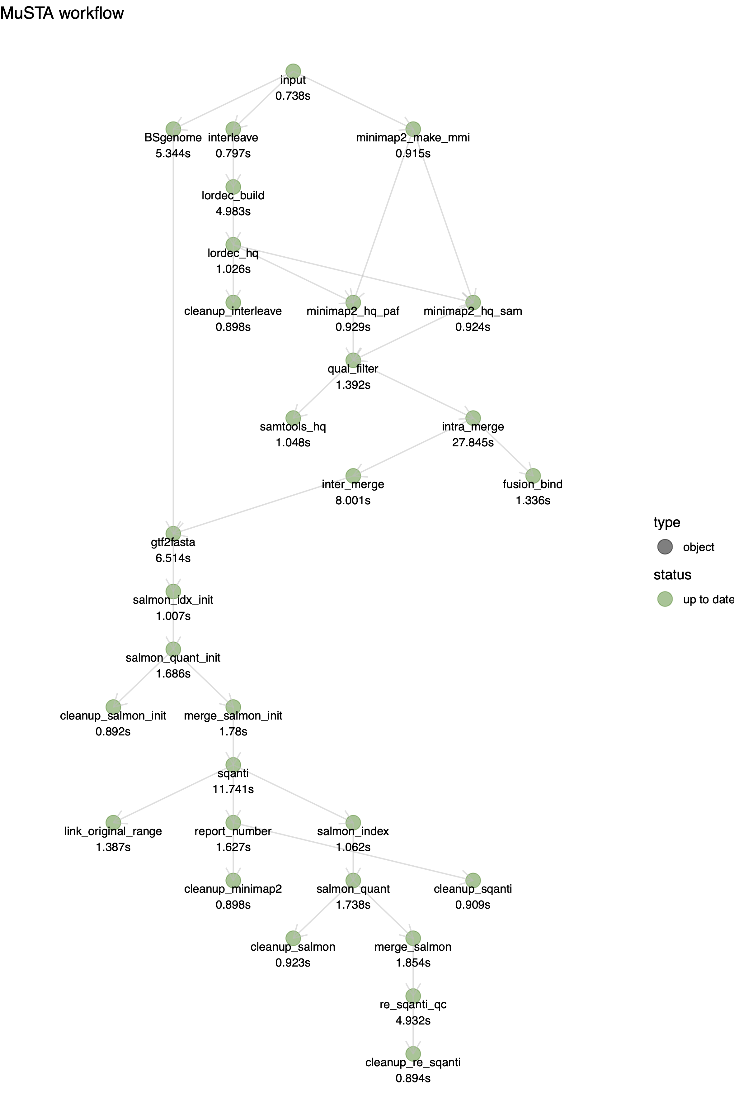plan_post_run

All of the important outputs can be found in the ‘result’ directory. The main outputs have the prefix supplied by the --prefix option (in this tutorial, the prefix is ‘musta’).

# The assembled transcriptome
## fasta
print(Biostrings::readDNAStringSet("test/test_output/result/musta.fa"))

#>   A DNAStringSet instance of length 8
#>     width seq                                          names               
#> [1]   571 TGGAGGAAAGATGAGTGAGAG...GAAAACAGGGGAATCCCGAA PB.1.1
#> [2]  1652 CTTGCCGTCAGCCTTTTCTTT...AAGCACACTGTTGGTTTCTG PB.1.2
#> [3]   248 CCTTTGGTTCTGCCATTGCTG...GAAAACAGGGGAATCCCGAA PB.1.3
#> [4]   920 CTTAGGGAACAAGCATTAAAC...TGAATTGATGTTTTCCTGCT PB.2.1
#> [5]   699 AGGGGCGCGCAGCGCCGGCGC...TTTTTGGAGATTTCTGTCTT PB.2.2
#> [6]  1800 AACTGAGGTCACCAGTCCCCA...GAGTGTCAGTTTAATGCTTG PB.3.1
#> [7]   567 GTAACACACAATACAGACTTC...ATATAAAAGATAGAAATCTC PB.4.1
#> [8]   207 AGAGCCTAGAAAATATCACCT...AAATACGCAAAATAAAGAGC PB.4.2

## gtf
knitr::kable(as.data.frame(rtracklayer::import("test/test_output/result/musta.gtf")))

seqnames	start	end	width	strand	source	type	score	phase	gene_id	transcript_id
18	11200	12999	1800	-	NA	exon	NA	NA	PB.3	PB.3.1
16	11861	11908	48	+	NA	exon	NA	NA	PB.1	PB.1.1
16	12294	12378	85	+	NA	exon	NA	NA	PB.1	PB.1.1
16	12663	12733	71	+	NA	exon	NA	NA	PB.1	PB.1.1
16	12906	13073	168	+	NA	exon	NA	NA	PB.1	PB.1.1
16	13153	13351	199	+	NA	exon	NA	NA	PB.1	PB.1.1
16	11555	11908	354	+	NA	exon	NA	NA	PB.1	PB.1.2
16	12294	12402	109	+	NA	exon	NA	NA	PB.1	PB.1.2
16	12902	14090	1189	+	NA	exon	NA	NA	PB.1	PB.1.2
16	13025	13073	49	+	NA	exon	NA	NA	PB.1	PB.1.3
16	13153	13351	199	+	NA	exon	NA	NA	PB.1	PB.1.3
18	14195	14653	459	-	NA	exon	NA	NA	PB.4	PB.4.1
18	14851	14958	108	-	NA	exon	NA	NA	PB.4	PB.4.1
18	14490	14653	164	-	NA	exon	NA	NA	PB.4	PB.4.2
18	16856	16898	43	-	NA	exon	NA	NA	PB.4	PB.4.2
18	11191	11595	405	+	NA	exon	NA	NA	PB.2	PB.2.1
18	13152	13354	203	+	NA	exon	NA	NA	PB.2	PB.2.1
18	15617	15928	312	+	NA	exon	NA	NA	PB.2	PB.2.1
18	11103	11595	493	+	NA	exon	NA	NA	PB.2	PB.2.2
18	15617	15822	206	+	NA	exon	NA	NA	PB.2	PB.2.2

## PBcount: the number of uniquely associated full-length non-chimeric (FLNC) reads
knitr::kable(readr::read_tsv("test/test_output/result/musta.pbcount.txt", col_types = readr::cols(.default = readr::col_character())))

gene_id	transcript_id	sample1	sample2	sample3	sample4
PB.1	PB.1.1	1	0	0	0
PB.1	PB.1.2	2	2	4	2
PB.1	PB.1.3	0	0	0	1
PB.2	PB.2.1	3	2	0	3
PB.2	PB.2.2	1	0	2	0
PB.3	PB.3.1	3	4	4	4
PB.4	PB.4.1	1	3	0	0
PB.4	PB.4.2	1	0	0	0

## (Short-read) expression: Transcript-per-Million (TPM) calclated by salmon
knitr::kable(read.table("test/test_output/result/musta.salmon.tpm.txt", header = TRUE, sep = "\t"))

	sample1	sample2	sample3	sample4
PB.1.1	1.511232e+04	44382.6210	88062.37451	1.472174e+04
PB.1.2	3.120952e+01	127.4420	21.76253	1.540468e+01
PB.1.3	0.000000e+00	0.0000	0.00000	0.000000e+00
PB.2.1	4.213970e-01	2571.9971	17.17896	4.783747e+00
PB.2.2	1.798816e+04	13003.6101	8130.36359	2.941479e+04
PB.3.1	6.512953e+04	482.1847	394043.41935	5.035502e+01
PB.4.1	1.461157e+00	44382.6210	221.16281	1.472174e+04
PB.4.2	9.017369e+05	895049.5241	509503.73825	9.410712e+05

You can conduct downstream analyses to investigate differentially expressed gene, differential transcript usage and so on. Most of the popular packages such as {DESeq2}, {DEXSeq}, and {SUPPA2} are available by setting the assembled transcriptome as reference. Some users might find tappas is useful for these purposes if they would like to conduct a number of analyses on GUI. The transcriptome can be imported to tappas with the aid of IsoAnnotLite.